
Modbus dates from 1979, and it is still everywhere: power meters, VFDs, flow computers, PLCs, and the gateways in front of RS-485 buses. It is also one of the least helpful protocols to read data from. There are no tag names, no data types and no units. A device exposes numbered 16-bit registers, and the meaning of each one lives in a PDF from the manufacturer.
So reading Modbus is mostly about the register map. Get the addresses, types, word order and scaling right, and the data is easy. Get one of them wrong, and you store numbers that look plausible and are not.
For this tutorial I built a small lab: a simulated three-phase power meter on Modbus TCP, read by Telegraf, stored in Arc, and queried with SQL for energy, power and voltage. Every command and query below was run against the lab, and the outputs are the real ones.
What the lab runs
| Component | Version |
|---|---|
| Arc | 26.09.4 (ghcr.io/basekick-labs/arc:26.09.4) |
| Telegraf | 1.40.3 (telegraf:1.40.3), with inputs.modbus and outputs.arc |
| Simulated meter | Python 3.12 with pymodbus 3.11.4 |
| arcli | 26.09.4 |
Telegraf's Arc output plugin ships with Telegraf 1.37 and later. The meter is pinned to pymodbus 3.11.4 on purpose. pymodbus 3.13.0 removed the datastore's setValues and rebuilt these classes on its new SimData/SimDevice API, so this script fails there; 3.12 still works.
Step 1: the register map
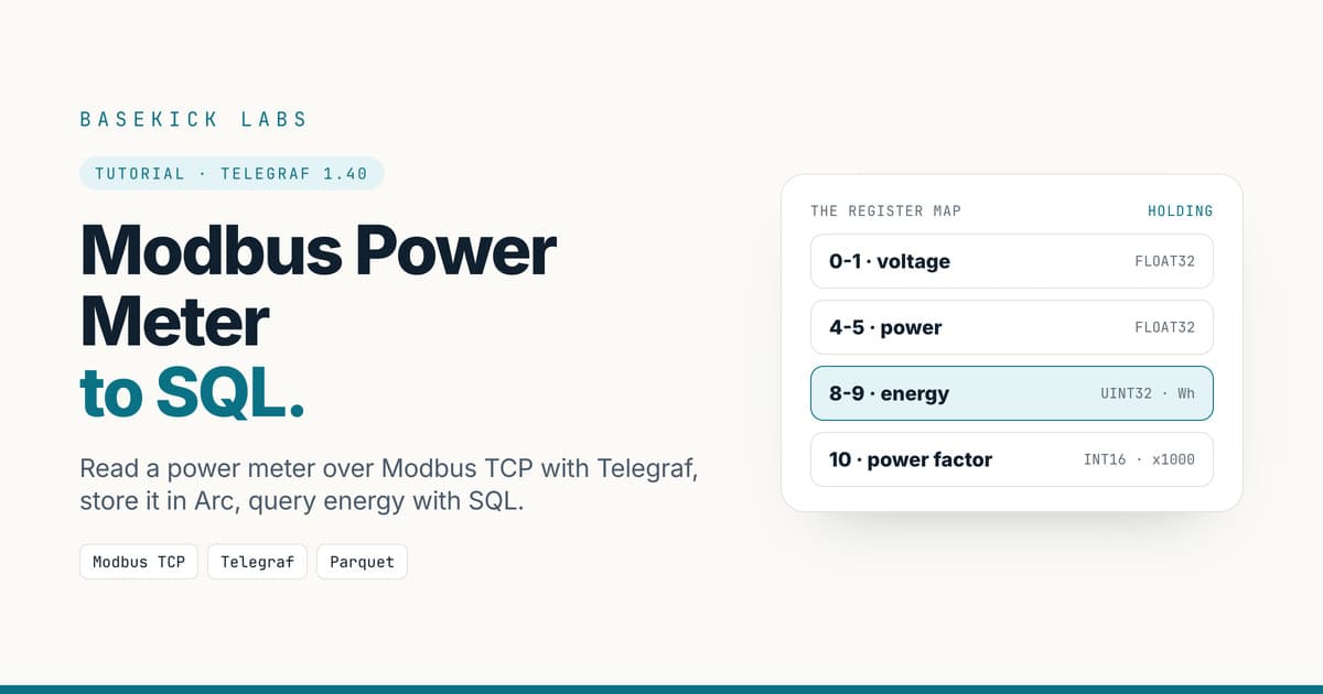
Every Modbus integration starts with a table like this one. Ours describes the simulated meter: holding registers, starting at address 0, big-endian.
| Address | Name | Type | Unit | Notes |
|---|---|---|---|---|
| 0-1 | voltage | FLOAT32 | V | line-to-neutral |
| 2-3 | current | FLOAT32 | A | |
| 4-5 | power | FLOAT32 | kW | three-phase active power |
| 6-7 | frequency | FLOAT32 | Hz | |
| 8-9 | energy | UINT32 | Wh | a counter that only goes up |
| 10 | power_factor | INT16 | x1000 | 930 means 0.930 |
Three details in there cause most Modbus problems:
- 32-bit values span two registers. A float or a 32-bit counter is split across two 16-bit registers, and devices disagree on which half comes first.
- Addresses are zero-based on the wire. Manuals often write holding registers as 40001, 40002 and so on. Register 40001 is address 0 in Telegraf. If every value looks shifted by one register, this is why.
- Scaling is in the manual, not the data. The meter sends
930for a power factor of 0.930 and watt-hours for energy. Nothing in the protocol tells you that.
If you have a real meter on the network, skip the simulator: point controller in step 4 at the meter's IP address and port (502 is the Modbus TCP default), and use its register map.
The simulator is a small Python script, meter.py. It keeps a slowly drifting voltage and current, computes power from them, and integrates power into the energy counter once a second:
"""A simulated three-phase power meter on Modbus TCP (port 5020, unit 1).

Holding registers, big-endian (ABCD):
  0-1   voltage       FLOAT32  V
  2-3   current       FLOAT32  A
  4-5   power         FLOAT32  kW
  6-7   frequency     FLOAT32  Hz
  8-9   energy        UINT32   Wh, a counter that only goes up
  10    power_factor  INT16    x1000
"""
import asyncio
import random
import struct

from pymodbus.datastore import (ModbusDeviceContext, ModbusSequentialDataBlock,
                                ModbusServerContext)
from pymodbus.server import StartAsyncTcpServer


def f32(value):  # one float -> two 16-bit registers, high word first
    return list(struct.unpack(">HH", struct.pack(">f", value)))


def u32(value):  # one unsigned 32-bit int -> two registers, high word first
    return [(value >> 16) & 0xFFFF, value & 0xFFFF]


async def update(device):
    voltage, current, energy_wh = 230.0, 40.0, 1_250_000.0
    while True:
        voltage += random.uniform(-0.4, 0.4) + (230.0 - voltage) * 0.05
        current = max(0.0, current + random.uniform(-2.0, 2.0) + (40.0 - current) * 0.05)
        pf = random.uniform(0.90, 0.97)
        power_kw = 3 * voltage * current * pf / 1000  # three phases, line-to-neutral
        energy_wh += power_kw * 1000 / 3600           # one second of energy
        values = (f32(voltage) + f32(current) + f32(power_kw)
                  + f32(50.0 + random.uniform(-0.03, 0.03))
                  + u32(int(energy_wh)) + [int(pf * 1000)])
        device.setValues(3, 0, values)                 # 3 = holding registers
        await asyncio.sleep(1)


async def main():
    device = ModbusDeviceContext(hr=ModbusSequentialDataBlock(0, [0] * 32))
    context = ModbusServerContext(devices=device, single=True)
    asyncio.create_task(update(device))
    await StartAsyncTcpServer(context=context, address=("0.0.0.0", 5020))


asyncio.run(main())
Step 2: the stack
Everything runs from one Compose file. The meter container installs pymodbus at start, so the only file it needs is meter.py.
services:
  meter:
    image: python:3.12-slim
    command: sh -c "pip install --quiet --root-user-action=ignore pymodbus==3.11.4 && python -u /app/meter.py"
    volumes:
      - ./meter.py:/app/meter.py:ro
    ports:
      - "5020:5020"

  arc:
    image: ghcr.io/basekick-labs/arc:26.09.4
    environment:
      ARC_AUTH_BOOTSTRAP_TOKEN: ${ARC_ADMIN_TOKEN}
    ports:
      - "8000:8000"
    volumes:
      - arc-data:/app/data

  telegraf:
    image: telegraf:1.40.3
    depends_on: [meter, arc]
    environment:
      ARC_TOKEN: ${TELEGRAF_TOKEN}
    volumes:
      - ./telegraf.conf:/etc/telegraf/telegraf.conf:ro

volumes:
  arc-data:
Create a .env next to it with a random admin token and an empty slot for Telegraf's. The slot is called TELEGRAF_TOKEN rather than ARC_TOKEN, because arcli reads an ARC_TOKEN environment variable of its own:
printf 'ARC_ADMIN_TOKEN=%s\nTELEGRAF_TOKEN=\n' "$(openssl rand -hex 24)" > .envStep 3: Arc and a write-only token
Start the meter and Arc, point arcli at Arc with the admin token, and create a token for Telegraf that can only write:
docker compose up -d meter arc
source .env
arcli config create --name modbus-lab --endpoint http://localhost:8000 --token "$ARC_ADMIN_TOKEN" --activate
arcli auth token create --name telegraf-meter --permission write \
  --description "Modbus collector, main incomer"
arcli prints the secret on stdout, once, followed by this on stderr:
Created token "telegraf-meter" (id 2). Store the secret securely; it cannot be retrieved again.Paste the secret into TELEGRAF_TOKEN= in .env and check what it can do:
source .env
arcli ping --endpoint http://localhost:8000 --token "$TELEGRAF_TOKEN"
arcli query --endpoint http://localhost:8000 --token "$TELEGRAF_TOKEN" "SHOW DATABASES"
endpoint: http://localhost:8000 (connection (flags))
health: ok (uptime 54m48.182500526s, latency 2.6ms) storage: hot=ok
auth: ok as "telegraf-meter" (id 2, write) — not admin; `auth token` commands will be refused
Error: arc: Permission denied: read required (HTTP 403)That is the token you want on a box that sits on the plant network. It can add data and nothing else. The OPC UA tutorial walks through this step in more detail.
Step 4: the Telegraf inputs.modbus config
This is the register map from step 1, written as Telegraf's request configuration:
[agent]
  interval = "5s"
  omit_hostname = true
  flush_interval = "10s"

[[inputs.modbus]]
  name = "meter"
  controller = "tcp://meter:5020"
  configuration_type = "request"

  [[inputs.modbus.request]]
    slave_id = 1
    byte_order = "ABCD"
    register = "holding"
    measurement = "power_meter"
    fields = [
      { address=0,  name="voltage",      type="FLOAT32" },
      { address=2,  name="current",      type="FLOAT32" },
      { address=4,  name="power_kw",     type="FLOAT32" },
      { address=6,  name="frequency",    type="FLOAT32" },
      { address=8,  name="energy_kwh",   type="UINT32", scale=0.001 },
      { address=10, name="power_factor", type="INT16",  scale=0.001 },
    ]
    [inputs.modbus.request.tags]
      site = "plant_a"
      meter = "main_incomer"

[[outputs.arc]]
  url = "http://arc:8000/api/v1/write/msgpack"
  api_key = "${ARC_TOKEN}"
  database = "plant"
  content_encoding = "gzip"
configuration_type = "request"lets you describe one Modbus read per block of registers. Telegraf reads all six fields here in one request: its log saysGot 1 request(s) touching 11 holding registers for 6 fields. Reading a block at once is faster and gentler on the device than one request per value.byte_order = "ABCD"means big-endian, high word first. That matches the meter. It's the setting to check first on a real device (see the next step).scaleturns the raw integers into engineering units: watt-hours into kilowatt-hours, and 930 into 0.930. Scaled fields come out asFLOAT64, as do theFLOAT32ones.- The tags (
site,meter) are what you will group and filter by in SQL. Put the meter's identity in tags, not in the measurement name. outputs.arcwrites MessagePack to Arc'splantdatabase with the write-only token.
Step 5: check byte order and scaling before you trust the values
Before starting the collector, run one read with --test. It prints what Telegraf decoded and sends nothing:
docker compose run --rm --no-deps telegraf telegraf --test> power_meter,meter=main_incomer,name=meter,site=plant_a,slave_id=1,type=holding_register current=34.59056091308594,energy_kwh=1251.88,frequency=49.97227478027344,power_factor=0.9520000000000001,power_kw=22.71816635131836,voltage=229.9092559814453 1794851380000000000These look right: 230 V, 50 Hz, and 3 × 229.9 V × 34.6 A × 0.952 ≈ 22.7 kW. Now here is the same read with the word order wrong, byte_order = "CDAB":
> power_meter,...,current=423919250709676000,energy_kwh=438829.075,frequency=-5764935722857080000000,power_factor=0.9520000000000001,power_kw=-0.4028450548648834,voltage=-7452395254362052000000000 1794851381000000000The voltage, current and frequency are absurd, so you would catch those. But look at the other two:
power_kwis -0.40. A meter on a line that exports a little power could report that. With the wrong word order, every float is effectively random on each poll; this read just happened to land somewhere believable.energy_kwhis 438,829. That's a perfectly believable reading for an energy counter. Only the deltas give it away: it climbs by about 65 kWh for every watt-hour the meter counts.
And power_factor is still correct, because it's a single 16-bit register and CDAB only swaps the two words of 32-bit values. With BADC or DCBA, the bytes inside each register swap too, and 16-bit values would be wrong as well. A wrong byte order doesn't always produce obvious garbage.
So check every 32-bit value against the device's own display or web page before you start collecting, and check one quantity you can derive from the others, as with power above. Real meters use all four orders (ABCD, CDAB, BADC, DCBA); the manual is the authority, and the display is the test.
Step 6: start collecting and look at what lands
docker compose up -d telegrafAfter a few minutes, query the newest rows with the admin connection:
arcli query "SELECT time, voltage, current, power_kw, energy_kwh, power_factor, site, meter
             FROM plant.power_meter ORDER BY time DESC LIMIT 3"
│ TIME │ VOLTAGE │ CURRENT │ POWER KW │ ENERGY KWH │ POWER FACTOR │ SITE │ METER │
│ 2026-11-16T18:39:45Z │ 229.44955444335938 │ 45.56993865966797 │ 28.828195571899414 │ 1273.253 │ 0.919 │ plant_a │ main_incomer │
│ 2026-11-16T18:39:40Z │ 229.98744201660156 │ 41.82444763183594 │ 26.15528678894043 │ 1273.214 │ 0.906 │ plant_a │ main_incomer │
│ 2026-11-16T18:39:35Z │ 230.06533813476562 │ 50.770782470703125 │ 32.61579895019531 │ 1273.173 │ 0.93 │ plant_a │ main_incomer │Each register became a typed column, and each tag became a column you can filter on.
Telegraf also adds three tags of its own: name (the inputs.modbus name), slave_id and type. They're useful once you poll several devices.
Scaled values can carry floating-point noise, such as 0.9530000000000001 for a power factor. Round them in queries, or add a processors.round step (Telegraf 1.36 and later) if you'd rather store rounded values.
Step 7: energy, demand and voltage in SQL
By the time I ran these queries, the lab had collected 614 readings over 51 minutes, one every 5 seconds.
Energy per interval: use the deltas
The obvious way to get energy per minute from a counter is the last reading minus the first, per minute:
SELECT time_bucket(INTERVAL '1 minute', time) AS minute,
       round(max(energy_kwh) - min(energy_kwh), 3) AS kwh
FROM plant.power_meter
GROUP BY minute
ORDER BY minute
It undercounts. Each minute holds 12 readings, so max - min covers 11 intervals and drops the one between the last reading of a minute and the first reading of the next. That's one interval in twelve.
The correct way is to compute the change between consecutive readings and add those up:
WITH deltas AS (
  SELECT time,
         energy_kwh - lag(energy_kwh) OVER (PARTITION BY site, meter ORDER BY time) AS kwh
  FROM plant.power_meter
)
SELECT time_bucket(INTERVAL '1 minute', time) AS minute,
       round(sum(kwh), 3) AS kwh
FROM deltas
GROUP BY minute
ORDER BY minute
Side by side, for ten minutes of the lab:
| Minute (UTC) | max − min | sum of deltas | avg kW |
|---|---|---|---|
| 18:20 | 0.370 | 0.404 | 24.21 |
| 18:21 | 0.374 | 0.408 | 24.79 |
| 18:22 | 0.383 | 0.410 | 25.52 |
| 18:23 | 0.425 | 0.463 | 28.03 |
| 18:24 | 0.386 | 0.424 | 25.29 |
| 18:25 | 0.404 | 0.438 | 26.20 |
| 18:26 | 0.395 | 0.432 | 26.15 |
| 18:27 | 0.426 | 0.461 | 27.81 |
| 18:28 | 0.373 | 0.407 | 24.55 |
| 18:29 | 0.410 | 0.445 | 26.92 |
The deltas agree with the power readings: 24.21 kW for one minute is 0.4035 kWh, and the deltas give 0.404. Across all 50 complete minutes of the lab, max - min added up to 19.542 kWh and the deltas to 21.291 kWh, so max - min was 8.2% low. On a monthly energy report, that's a real number.
Counters do reset: a meter is replaced, or its register rolls over. When that happens, the delta for one row is a large negative number. The lab had none, but in production, filter them out with WHERE kwh >= 0 in the outer query, or handle resets explicitly if you bill from this data.
Demand: the average over the interval, not the peak
Utilities bill demand as the highest average power over their demand interval, often 15 minutes. That's a different number from the highest reading:
SELECT time_bucket(INTERVAL '15 minutes', time) AS interval_start,
       count(*) AS readings,
       round(avg(power_kw), 2) AS demand_kw,
       round(max(power_kw), 2) AS instant_peak_kw
FROM plant.power_meter
GROUP BY interval_start
ORDER BY interval_start
│ INTERVAL START │ READINGS │ DEMAND KW │ INSTANT PEAK KW │
│ 2026-11-16T17:45:00Z │ 136 │ 25.32 │ 31.05 │
│ 2026-11-16T18:00:00Z │ 180 │ 25.25 │ 30.65 │
│ 2026-11-16T18:15:00Z │ 180 │ 26.03 │ 32.89 │
│ 2026-11-16T18:30:00Z │ 118 │ 26.15 │ 32.62 │The first and last intervals are partial (180 readings is a full 15 minutes at 5 seconds). Of the complete intervals, the highest demand was 26.03 kW, while the highest single reading in that interval was 32.89 kW. Reporting the instantaneous peak as demand would overstate it by about a quarter.
Voltage outside a band
SELECT count(*) AS readings,
       count(*) FILTER (WHERE voltage NOT BETWEEN 229 AND 231) AS outside_229_231,
       round(min(voltage), 2) AS v_min,
       round(max(voltage), 2) AS v_max
FROM plant.power_meter
│ READINGS │ OUTSIDE 229 231 │ V MIN │ V MAX │
│ 614 │ 127 │ 227.79 │ 232.14 │The band here is tight so that the simulator trips it. In practice you would use your supply's tolerance, and drop the aggregate to list the excursions themselves with their timestamps.
Before production
What I would change from this lab before pointing it at real equipment:
- Confirm the map against the device. Check every 32-bit value against the display, and one derived quantity (power from volts, amps and power factor), before you trust a week of data.
- Poll at the rate the process needs. Energy meters are fine at 5 to 60 seconds. Many devices, especially behind RS-485 gateways, cope badly with fast polling. Telegraf's
busy_retriesoption andpause_between_requests(in the[inputs.modbus.workarounds]table) help with slow or busy devices. - Use RTU when the device is on a serial bus. The same plugin reads Modbus RTU or ASCII over serial (
controller = "file:///dev/ttyUSB0", withbaud_rateand friends), and RTU over TCP through gateways. - Keep the Arc token write-only, and put TLS in front of Arc if the path crosses a network you don't fully control.
- Raise the flush interval to cut the number of small Parquet files written between compactions.
Wrapping up
Once the register map is right and checked against the device, Modbus data is typed columns in SQL, stored as Parquet you own.
If your plant speaks OPC UA rather than Modbus, see OPC UA to SQL with Telegraf. If your devices publish over MQTT, Arc can subscribe to the broker directly. If you need logic between the register and the database, Node-RED can write to Arc too. And if per-tag licensing is the reason you log fewer signals than you'd like, read why your historian charges per tag. The Telegraf integration docs cover the Arc output plugin.