
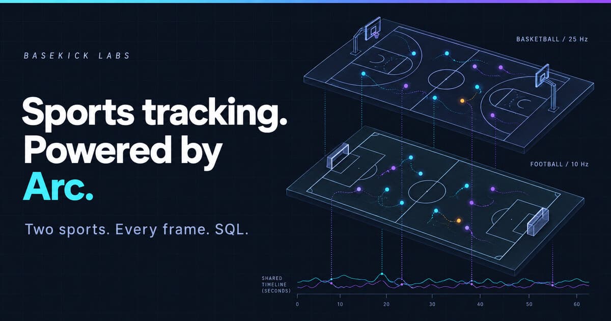
Ten players and a ball, 25 positions a second each, for a whole NBA game. Twenty-two players and a ball, ten positions a second, for a whole football match. Nobody thinks of a basketball court as a sensor network, but that is what optical tracking turns it into, and the questions people ask of it are time-series questions: where was this player at this instant, how fast were they moving, who was closest, what did the ball do during that shot.
We built two demos to make that visible.
NBA Player Tracking replays Cleveland at Golden State from 25 December 2015, reconstructed from SportVU tracking data. Soccer Player Tracking replays Melbourne Victory against Auckland FC from May 2025, reconstructed from SkillCorner's open broadcast tracking. Both run on the same Arc instance as our other live demos.
This post covers what you see on the page, what is going on underneath, and then the part that matters for teams: what a club can do with its own training and match data on Arc.
What the demo shows
Press play and the court fills with dots moving the way the players moved. Drag the scrubber to any second of the game. Click a player and the panel next to the court fills with their position, speed, distance covered and nearest opponent, while three charts under the court track speed, separation and ball height along the playhead.
The panel labelled Arc query is the point of the exercise. It shows the exact SQL the page sent to Arc to draw the frame you are looking at, the number of rows that came back, and the time Arc took to run it. Not round trip, not API overhead: the engine time Arc reports on its own query response. Seek somewhere else and the query changes. Select a player and two more queries appear.
Every number on the page carries one of three labels. Raw telemetry is a stored observation. Arc query was computed inside the database, and the SQL is right there. Derived client metric was computed in the browser from the observations it had already buffered. We show client-side and Arc-side versions of the same quantity side by side on purpose, so you can see that they agree and decide for yourself where a calculation belongs.
Some measured figures from the import, read back from Arc rather than typed:
| NBA game | Football match | |
|---|---|---|
| Sampling rate | 25 Hz | 10 Hz |
| Frames stored | 85,450 | 40,404 |
| Observations (rows) | 939,454 | 929,292 |
| Tracked play | 57 minutes | 67 minutes |
The NBA source file had 233,039 frames, of which 147,589 were duplicates: the data is organized around play-by-play events, and adjacent events repeat each other's frames. The importer keys frames on capture time, verifies that repeated keys carry identical positions, and keeps one copy. That kind of cleanup is most of the work in any tracking pipeline, and it is documented on the demo page.
What is underneath
The schema is deliberately plain. One row per entity per frame:
tracking(time, game_id, period, game_clock, shot_clock, event_id,
         frame_seq, entity_type, team_id, player_id, x, y, z)
time is the real capture timestamp SportVU stamps on every frame. Period, game clock and shot clock sit next to it as ordinary columns, so nothing sporting is lost and every query is still a time-range query. Playback asks for bounded windows:
SELECT epoch_ms(time) AS t, period, game_clock, shot_clock, event_id,
       entity_type, team_id, player_id, x, y, z
FROM tracking
WHERE game_id = '0021500438'
  AND time >= TIMESTAMP '2015-12-25 22:20:35.065'
  AND time <  TIMESTAMP '2015-12-25 22:20:55.065'
ORDER BY time, entity_type, player_id
Twenty seconds of every entity, about 5,500 rows, and the browser prefetches the next window while this one plays. Speed is a window function over one player's rows:
WITH p AS (
  SELECT time, x, y FROM tracking
  WHERE game_id = '0021500438' AND player_id = 201939
    AND time >= TIMESTAMP '2015-12-25 22:20:35.065'
    AND time <  TIMESTAMP '2015-12-25 22:20:55.065'
)
SELECT epoch_ms(time) AS t, x, y,
       sqrt(power(x - LAG(x) OVER (ORDER BY time), 2)
          + power(y - LAG(y) OVER (ORDER BY time), 2))
       / ((epoch_ms(time) - LAG(epoch_ms(time)) OVER (ORDER BY time)) / 1000.0) AS speed_fps
FROM p ORDER BY time
Nearest defender is a self-join at equal timestamps, reduced with arg_min:
WITH me  AS (SELECT time, x, y FROM tracking WHERE player_id = 201939 AND ...),
     opp AS (SELECT time, player_id, x, y FROM tracking
             WHERE entity_type = 'player' AND team_id <> 1610612744 AND ...),
     pairs AS (
       SELECT me.time, opp.player_id,
              sqrt(power(me.x - opp.x, 2) + power(me.y - opp.y, 2)) AS dist
       FROM me JOIN opp ON opp.time = me.time
     )
SELECT epoch_ms(time) AS t, arg_min(player_id, dist) AS nearest, min(dist) AS distance_ft
FROM pairs GROUP BY time ORDER BY time
On the demos instance these run in tens of milliseconds over the 20-second window: 26 ms for the speed query and 48 ms for the nearest-defender join when we measured them while building the page. Downsampling a whole quarter of ball height to one row per second is a time_bucket:
SELECT time_bucket(INTERVAL 1 SECOND, time) AS bucket,
       max(z) AS max_height_ft, avg(z) AS avg_height_ft
FROM tracking
WHERE game_id = '0021500438' AND entity_type = 'ball' AND period = 1
GROUP BY 1 ORDER BY 1
Standard SQL, no proprietary query language, and the data on disk is Parquet you can open with DuckDB, pandas or Spark without asking Arc's permission. The football demo uses the same components with a different renderer and a different coordinate system. Adding a third sport is an importer and a config file.
What this means for a team
A professional club generates the same shape of data every day, from more sources than the demo uses:
- Training: GPS or LPS wearables at 10 to 100 Hz per player, with accelerometer and gyroscope channels on top of position.
- Matches: optical tracking from the league or a provider, at 10 to 25 Hz, plus event data (passes, shots, pressures) that has to line up with it.
- Everything else: heart rate, wellness questionnaires, sleep, load scores, video timestamps.
A season of that runs to billions of observations for a single squad. The workflow most clubs live with is a pile of vendor exports and CSVs, one notebook per question, and a data scientist who spends more time joining files than answering the coach.
Put the raw observations in a time-series database instead and the questions become queries the whole staff can run, on a shared, up-to-date dataset:
Load management. Distance, high-speed running, accelerations and decelerations per session, per player, rolled up by day and by week. With time_bucket and window functions, the acute-to-chronic workload ratio is one query, not a spreadsheet. Assuming a wearables measurement with per-sample speed and distance columns:
WITH daily AS (
  SELECT time_bucket(INTERVAL 1 DAY, time) AS day, player_id,
         sum(distance_m) FILTER (WHERE speed_mps > 5.5) AS hsr_m
  FROM wearables
  WHERE time > now() - INTERVAL 35 DAY
  GROUP BY 1, 2
)
SELECT day, player_id,
       sum(hsr_m) OVER (PARTITION BY player_id ORDER BY day ROWS 6 PRECEDING)  AS acute_7d,
       avg(hsr_m) OVER (PARTITION BY player_id ORDER BY day ROWS 27 PRECEDING) * 7 AS chronic_28d
FROM daily
ORDER BY day DESC, player_id
Tactical analysis. Team compactness, line heights, pressing distance to the ball carrier, time to close down: all of them are distance and speed calculations over the tracking rows, exactly like the nearest-defender query above, aggregated by phase of play.
Opponent scouting. The same queries against opposition matches, because the schema does not care whose team it is.
Individual development. A player's top speed and repeat-sprint profile across two seasons, from one table, with the raw samples still there when someone questions a number.
Rehabilitation. Progression of a returning player's load against their own pre-injury baseline, day by day.
The common thread: keep the raw observations, at full resolution, in one place where SQL reaches them. Aggregates are cheap to recompute. Raw data you threw away is gone.
Start with Arc OSS
Everything in the demos runs on Arc's open-source edition. A single node handles a squad's worth of tracking without effort; the demos instance holds both games alongside every other live demo on the site. To try it with your own data:
docker run -d -p 8000:8000 \
  -e STORAGE_BACKEND=local \
  -v arc-data:/data \
  ghcr.io/basekick-labs/arc:latest
Ingest from Python with the MessagePack columnar endpoint (that is how the demo importers write), from any InfluxDB line protocol client, or from Telegraf. Query over HTTP with SQL, or through Arrow for large results. Point Grafana at it. Read the Parquet directly from a notebook when you want to train a model.
The NBA importer is a few hundred lines of Python: download, deduplicate, batch, write, verify. A club's importer for a wearable export or a tracking-provider feed looks the same.
Expand with Arc Enterprise
Arc Enterprise is the same binary; a license key turns on the features a club needs once tracking data becomes shared infrastructure rather than one analyst's project.
Access control. Player tracking is personal data, and medical and wellness data more so. Enterprise adds organizations, teams and roles with permissions down to the measurement, so the medical staff see wellness data, the analysts see tracking, the academy sees the academy, and a departing staff member's token stops working the day they leave. Audit logging records who queried what, which is the question a data protection officer asks first.
One store for the whole club. Clustering with separate writer, reader and compactor roles keeps a heavy match-day ingest from slowing down the coaches' dashboards, with automatic failover so nobody is paged during a game.
Seasons that stay queryable. Tiered storage moves last season's raw samples to cold object storage automatically, on a per-database policy, and they stay queryable. Backup and restore is built in.
Numbers that are ready before the meeting. Continuous queries and retention policies exist in OSS; Enterprise schedules them. Per-session and per-week aggregates land in their own measurements overnight, so the morning report is a SELECT, not a job someone has to remember to run.
Shared without surprises. Query governance sets per-token rate limits, quotas and row caps, so an exploratory notebook cannot starve the match-day dashboard.
Tier I starts at $5,000 a year for a single server and can be bought online. Air-gapped and on-premises deployments are supported; the license validates locally. If you would rather not run it, Arc Enterprise Managed is the same product operated by us on dedicated hardware.
Try it
Open the NBA demo, press play, select a player, and read the SQL. Then open the football demo and notice it is the same query shapes on a different sport. If you work with tracking data and want to talk through what a season of it looks like on Arc, the form on either demo page reaches us directly, or write to enterprise@basekick.net.
Tracking data credits: NBA SportVU 2015-16 season as published in the NBA-Player-Movements repository; SkillCorner Open Data (MIT license). Neither dataset is redistributed by Basekick Labs.