
A vibration sensor at 20 kHz produces more data in one second than a temperature sensor does in a day. That single fact shapes how most condition monitoring systems are built: compute an RMS value at the edge, keep one number per minute, throw the waveform away. It keeps the database small. It also means that when a bearing finally fails, the one question everyone asks, what did the spectrum look like the hour before, has no data behind it.
We built a demo around the alternative: keep every sample.
Bearing Run to Failure replays NASA's IMS bearing test. Four Rexnord ZA-2115 bearings on a shaft at 2000 rpm under a 6000 lbs radial load, accelerometers on each housing sampled at 20 kHz, one second recorded every ten minutes for six days and twenty hours, until the outer race of bearing 1 fails. Every sample of every channel is a row in Arc.
What the demo shows
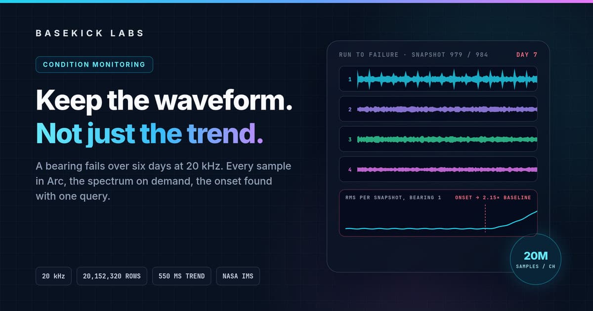
Press play and four waveforms step through the run at a few snapshots per second. For the first five days they look like noise, because they are: healthy bearings under load. Around day five the trace for bearing 1 starts to thicken. By the last morning its RMS is ten times what it was on day one, and the two final snapshots go flat because the rig has been stopped.
Pause anywhere and the page fetches the 20,480 raw samples of the selected bearing, draws them in place of the envelope, and computes the spectrum in the browser. Markers show the frequencies the bearing geometry predicts for each kind of damage: outer race, inner race, roller, cage, shaft. Pause on day six and the outer race frequency and its harmonics stand out of the floor. Pause on day two and they are not there. That is the whole story of the dataset, and you can scrub back and forth to find the snapshot where it begins.
The trend charts under the waveforms are the timeline. They hold RMS and kurtosis for all four bearings across the run, and clicking a point jumps the playback there. A jump to onset button goes to the first snapshot where bearing 1 exceeds twice its day-one baseline, which Arc finds with a window query.
Every number on the page carries one of the three labels we use on all the Arc demos. Raw telemetry is a stored observation. Arc query was computed in the database, and the SQL is in the panel next to the charts with Arc's own execution time. Derived client metric was computed in the browser from raw samples it fetched. The spectrum is client-side, and the inspector shows the browser's RMS next to Arc's for the same window so you can see them agree.
Measured figures, read back from the import rather than typed:
| Rows in Arc (per channel) | 20,152,320 |
| Snapshots | 984, one second every ten minutes |
| Run length | 163.8 hours |
| Size on disk | 306 MB |
| Import time | about two minutes, 123 write requests |
| Bearing 1 RMS, day one | 0.074 g |
| Bearing 1 RMS, final hour | 0.725 g |
What is underneath
The schema is one row per sample, one column per accelerometer, because that is how a data acquisition card writes and it makes a per-sensor query a column selection:
vibration(time, test_id, snapshot, sample, b1, b2, b3, b4)time is the file's timestamp plus 50 microseconds per sample, stored at microsecond precision. The snapshot and sample ordinals sit next to it so a snapshot can be addressed without timestamp arithmetic.
The trend charts come from one query over every row. It buckets the run into the ten-minute snapshots and computes RMS, peak and kurtosis per bearing:
SELECT time_bucket(INTERVAL 10 MINUTE, time) AS bucket,
       min(snapshot) AS snapshot,
       count(*) AS samples,
       sqrt(avg(b1 * b1)) AS rms_b1, max(abs(b1)) AS peak_b1, kurtosis(b1) AS kurt_b1,
       sqrt(avg(b2 * b2)) AS rms_b2, max(abs(b2)) AS peak_b2, kurtosis(b2) AS kurt_b2,
       sqrt(avg(b3 * b3)) AS rms_b3, max(abs(b3)) AS peak_b3, kurtosis(b3) AS kurt_b3,
       sqrt(avg(b4 * b4)) AS rms_b4, max(abs(b4)) AS peak_b4, kurtosis(b4) AS kurt_b4
FROM vibration
WHERE test_id = 'ims-2'
GROUP BY bucket
ORDER BY bucket
984 rows out of 20,152,320, in 552 ms on the demos instance when we measured it. Kurtosis is the interesting one: Gaussian noise gives 3, and impacts from a spalled race push it up before the RMS moves much.
Onset is the same aggregation in a CTE with a baseline over the first day:
WITH s AS (
  SELECT time_bucket(INTERVAL 10 MINUTE, time) AS bucket,
         min(snapshot) AS snapshot,
         sqrt(avg(b1 * b1)) AS rms
  FROM vibration
  WHERE test_id = 'ims-2'
  GROUP BY bucket
),
base AS (
  SELECT avg(rms) AS baseline
  FROM s
  WHERE bucket < (SELECT min(bucket) FROM s) + INTERVAL 1 DAY
)
SELECT s.snapshot, s.rms, base.baseline, s.rms / base.baseline AS ratio
FROM s, base
WHERE s.rms > 2 * base.baseline
ORDER BY s.bucket
LIMIT 1
It returns snapshot 702, about 47 hours before the end of the run, at 2.15 times baseline. 286 ms.
The waveforms during playback are not the raw samples; sending 20,480 points per channel eight times a second would be wasteful. They are a min/max envelope per millisecond, which is a time_bucket at a resolution most people do not associate with a time-series database:
SELECT snapshot,
       time_bucket(INTERVAL 1 MILLISECOND, time) AS ms,
       min(b1) AS lo_b1, max(b1) AS hi_b1,
       min(b2) AS lo_b2, max(b2) AS hi_b2,
       min(b3) AS lo_b3, max(b3) AS hi_b3,
       min(b4) AS lo_b4, max(b4) AS hi_b4
FROM vibration
WHERE test_id = 'ims-2'
  AND snapshot BETWEEN 700 AND 707
GROUP BY snapshot, ms
ORDER BY snapshot, ms
Eight snapshots, 8,192 rows, 146 ms. When you pause, the raw window for one channel is a plain range scan, 20,480 rows in about 110 ms, and the browser does the FFT.
Standard SQL throughout. The data on disk is Parquet, so the same 20 million rows are readable from DuckDB, pandas or Spark without going through Arc at all.
What this means for a plant
A single vibration point on a critical asset is exactly this workload. A plant has hundreds: gearboxes, pumps, fans, spindles, each with two or three accelerometers, plus the slow signals around them: temperature, current, speed, load, plus the maintenance events that give the numbers meaning.
The conventional pipeline keeps a handful of scalar features per sensor per interval and discards the rest at the edge. It works until someone wants a question the features cannot answer:
- Was this failure visible earlier? With raw waveforms kept, you can run today's detector across last year's data and find out at what point it would have fired. With features only, you can run it on nothing.
- Is this the same fault as the one on line 3 in March? Compare spectra of the two events. Features from two different vendor boxes rarely line up well enough for that.
- What does the new feature look like on old data? Crest factor, spectral kurtosis, a band energy at the gear mesh frequency: all of them are one query over the stored samples, backfilled across the whole history in one pass, the way the demo computes kurtosis over 20 million rows in half a second.
- Which sensors are lying? A stuck or saturating accelerometer is obvious in the raw signal and invisible in a well-behaved RMS.
The queries are the ones in the demo with a machine dimension added. Hourly RMS per sensor across the plant:
SELECT time_bucket(INTERVAL 1 HOUR, time) AS hour, machine_id, sensor,
       sqrt(avg(accel * accel)) AS rms_g,
       kurtosis(accel) AS kurt
FROM vibration
WHERE time > now() - INTERVAL 30 DAY
GROUP BY 1, 2, 3
ORDER BY 1, 2, 3
Every sensor currently above twice its own 30-day baseline, which is the onset query turned into a fleet-wide alert list:
WITH hourly AS (
  SELECT time_bucket(INTERVAL 1 HOUR, time) AS hour, machine_id, sensor,
         sqrt(avg(accel * accel)) AS rms_g
  FROM vibration
  WHERE time > now() - INTERVAL 30 DAY
  GROUP BY 1, 2, 3
),
scored AS (
  SELECT *,
         avg(rms_g) OVER (PARTITION BY machine_id, sensor ORDER BY hour ROWS 719 PRECEDING) AS baseline_30d
  FROM hourly
)
SELECT machine_id, sensor, hour, rms_g, rms_g / baseline_30d AS ratio
FROM scored
QUALIFY hour = max(hour) OVER (PARTITION BY machine_id, sensor)
   AND ratio > 2
ORDER BY ratio DESC
Storage is the objection people raise first, so here is the arithmetic from the demo: 20 million samples per channel, four channels, 306 MB on disk. That is about 3.8 bytes per sample. A sensor recording one second every ten minutes at 20 kHz all year is about 1.1 billion samples, roughly 4 GB at that ratio. A plant with 300 sensors is a bit over a terabyte a year of raw waveforms, on object storage, with the full history queryable. That is a smaller line item than the one visit from the failure the waveforms would have predicted.
Start with Arc OSS
Everything in the demo runs on Arc's open-source edition on a single node. To try it with a sensor of your own:
docker run -d -p 8000:8000 \
  -e STORAGE_BACKEND=local \
  -v arc-data:/data \
  ghcr.io/basekick-labs/arc:latest
The demo importer writes with the MessagePack columnar endpoint: 8 snapshots per request, 163,840 rows and about 9 MB each, 20 million rows in two minutes over a single connection. Historians and gateways that speak InfluxDB line protocol or Telegraf work unchanged, and MQTT subscriptions are built in. Query over HTTP with SQL, or through Arrow when you want 20,480 rows back fast. Point Grafana at it for the plant floor and open the Parquet from a notebook for the model work.
Expand with Arc Enterprise
Arc Enterprise is the same binary with a license key, and the features it adds are the ones a plant asks for once vibration data stops being one engineer's project.
One store per plant, not per line. Clustering with separate writer, reader and compactor roles, on shared object storage or on local disks with peer replication, so a burst of waveforms from the whole floor at shift change does not slow the maintenance planner's dashboard. Automatic failover, and cluster traffic under TLS.
OT and IT in the same database. Organizations, teams and roles with permissions down to the measurement: the reliability team sees vibration, the process engineers see their lines, the vendor doing a remote diagnosis gets a token scoped to one machine for one week. Audit logging records who read what, which matters the moment the data covers a safety-relevant asset.
Raw for a quarter, features forever. Tiered storage moves raw waveforms to cold object storage on a per-database policy while they stay queryable. Continuous queries and retention policies exist in OSS; Enterprise schedules them, so hourly RMS, kurtosis and band energies land in their own measurement every night and the raw samples age out on a schedule you set. Backup and restore are built in.
Shared without surprises. Query governance sets per-token rate limits, quotas and row caps, so a data scientist's notebook scanning a year of waveforms does not starve the alerting queries.
Tier I starts at $5,000 a year for one server and can be bought online. Air-gapped plants are supported; the license validates locally with no internet required. Arc Enterprise Managed is the same product operated by us on dedicated hardware if you would rather not run it.
Try it
Open the bearing demo, press play, wait for day five, pause and read the spectrum. Then open the query panel and see that everything you looked at was SQL. If you have vibration data of your own and want to know what a year of it looks like in Arc, the form on the demo page reaches us directly, or write to enterprise@basekick.net.
Data credit: IMS Bearing Data, NSF I/UCR Center for Intelligent Maintenance Systems, University of Cincinnati, with support from Rexnord Corp., distributed by the NASA Prognostics Center of Excellence data repository. Reference: Qiu, Lee and Lin, Journal of Sound and Vibration 289 (2006). Public domain; not redistributed by Basekick Labs.