Anomaly Detection on Sensor Data with Arc, in Pure SQL
A pump bearing doesn't fail all at once. It starts as a few extra hundredths of a millimeter of vibration, buried under the daily thermal swing, lost in sensor noise, invisible on a dashboard that's showing you a year of data zoomed to fit. For five days it climbs. Nobody's watching that one tag out of ten thousand. Then it seizes on a Tuesday night, takes the line down, and the post-mortem finds the warning was sitting in the historian the whole time. The data saw it coming. Nothing was looking.
That's the real problem with anomaly detection. It isn't the math, which is decades old. It's having a system that can run the math continuously, over every tag, cheaply enough that you actually do it. Most teams don't, because the usual answer is "export the data to Python, fit a model, stand up a service to score it." That's three new systems to operate before you've caught a single fault. So it never ships, and the bearing seizes on schedule.
This post takes the other path. Arc runs a full analytical SQL dialect over your Parquet data, which means the three workhorse detection methods (rolling z-score, robust MAD, and seasonal-residual) are each a single query Arc pushes down to the storage engine. No export, no model server, no second system. And with Continuous Queries, that single query becomes a standing detector watching every tag, all the time.
We'll build all three against a realistic dataset of 3.1 million vibration readings across three machines over 60 days, with two faults deliberately injected so we have something real to catch. One of them is exactly the slow bearing creep above. Every query here ran against a live Arc instance, and the charts are rendered from the actual results.
The data
Three machines (pump-01, pump-02, compressor-01) reporting vibration (mm/s) every 5 seconds for 60 days. The clean signal is a baseline around 4.5 mm/s with a daily thermal cycle and an 8-hour shift cycle, plus sensor noise. Into that we injected two faults:
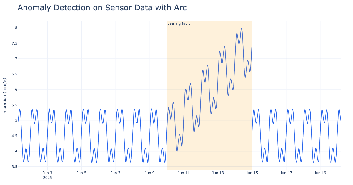
compressor-01: a sudden 6-hour excursion to ~11 mm/s on May 31 (think: a valve event).pump-01: a gradual bearing degradation over June 10 to 15, ramping from 4.5 up to ~7.5 mm/s, then snapping back after a repair.
The schema in Arc is just a measurement with a time column, a machine tag, and a value field. Ingestion is over Arc's binary MessagePack endpoint, and 3.1M rows land in under 2 seconds.
-- what we're working with
SELECT machine, count(*) AS readings,
       round(avg(value), 2) AS avg_vib,
       round(max(value), 2) AS max_vib
FROM vibration
GROUP BY machine;
Method 1: Rolling z-score
The classic. For each point, compute how many standard deviations it sits from a trailing window's mean. The textbook threshold is ±3σ; here we filter at ±4σ to cut false positives on noisy industrial signals (tune it to your data). In Arc this is one window function, and the key detail is the frame: ROWS BETWEEN 144 PRECEDING AND 1 PRECEDING means "the last 144 points before this one," so the current point can't pull its own baseline toward itself.
WITH series AS (
  SELECT machine,
         time_bucket(INTERVAL '10 minutes', time) AS ts,
         avg(value) AS v
  FROM vibration
  GROUP BY machine, ts
),
z AS (
  SELECT machine, ts, v,
         avg(v)    OVER w AS mean,
         stddev(v) OVER w AS sd
  FROM series
  WINDOW w AS (
    PARTITION BY machine ORDER BY ts
    ROWS BETWEEN 144 PRECEDING AND 1 PRECEDING
  )
)
SELECT machine, ts, v, (v - mean) / NULLIF(sd, 0) AS zscore
FROM z
WHERE abs((v - mean) / NULLIF(sd, 0)) > 4
ORDER BY abs((v - mean) / NULLIF(sd, 0)) DESC;
This runs in ~280 ms over the full 60 days. It cleanly flags the compressor event (z = 11.6 at the spike onset) and the end of the pump fault. That snap back to baseline registers as a large negative z-score (z = −5.3), because relative to the elevated trailing window, the return to 4.5 mm/s is itself an outlier. That's a feature, not a bug: step-changes in both directions are anomalies.
The shaded band is the injected fault. The red ×s are points the z-score flagged. Notice what rolling z-score is good at (sharp changes) and what it struggles with (the slow middle of the ramp, where the trailing window slowly adapts to the drift and stops seeing it as anomalous). Hold that thought, because Method 3 fixes exactly that.
Method 2: Robust MAD (median absolute deviation)
Mean and standard deviation have a weakness: a single huge spike inflates the standard deviation, which raises your detection threshold and can mask nearby real anomalies. The robust fix is to replace mean with median and stddev with MAD (median absolute deviation). The 0.6745 factor scales MAD to be comparable to a standard-deviation z-score for normally-distributed data.
One gotcha worth calling out: Arc's SQL engine won't let you nest median() OVER w inside another windowed median() in the same SELECT. Split it into two CTEs, computing the rolling median first, then the rolling MAD off of it:
WITH series AS (
  SELECT machine,
         time_bucket(INTERVAL '10 minutes', time) AS ts,
         avg(value) AS v
  FROM vibration
  GROUP BY machine, ts
),
with_median AS (
  SELECT machine, ts, v,
         median(v) OVER w AS med
  FROM series
  WINDOW w AS (PARTITION BY machine ORDER BY ts
              ROWS BETWEEN 144 PRECEDING AND 1 PRECEDING)
),
with_mad AS (
  SELECT machine, ts, v, med,
         median(abs(v - med)) OVER w AS mad
  FROM with_median
  WINDOW w AS (PARTITION BY machine ORDER BY ts
              ROWS BETWEEN 144 PRECEDING AND 1 PRECEDING)
)
SELECT machine, ts, v,
       0.6745 * (v - med) / NULLIF(mad, 0) AS robust_z
FROM with_mad
WHERE abs(0.6745 * (v - med) / NULLIF(mad, 0)) > 5
ORDER BY ts;
MAD brackets the entire compressor fault window cleanly, and because it doesn't let the spike inflate its own threshold, it stays sensitive on either side of the event. Use MAD when your signal has occasional transient glitches you don't want desensitizing your detector.
Method 3: Seasonal residual
The rolling methods share a blind spot: a slow drift. As a fault ramps up over days, the trailing window slowly follows it and the deviation shrinks, so the detector "gets used to" the new normal. You saw this in the middle of the pump ramp in Method 1.
The fix is to compare against a seasonal baseline, the expected value for this hour-of-day learned from a known-good period, instead of a trailing window. Drift can't hide from a fixed baseline.
WITH hourly AS (
  SELECT time_bucket(INTERVAL '1 hour', time) AS ts, avg(value) AS v
  FROM vibration
  WHERE machine = 'pump-01'
  GROUP BY ts
),
baseline AS (             -- expected value per hour-of-day, from the clean period
  SELECT extract('hour' FROM ts) AS hod,
         avg(v) AS expected,
         stddev(v) AS expected_sd
  FROM hourly
  WHERE ts < TIMESTAMP '2025-05-31'   -- training window (known good)
  GROUP BY hod
)
SELECT h.ts, h.v, b.expected,
       (h.v - b.expected) / NULLIF(b.expected_sd, 0) AS residual_z
FROM hourly h
JOIN baseline b ON extract('hour' FROM h.ts) = b.hod
WHERE abs((h.v - b.expected) / NULLIF(b.expected_sd, 0)) > 3
ORDER BY h.ts;
This is where seasonal residual earns its keep. As the bearing fault ramps, the residual z-score climbs monotonically, hitting 3, then 9, then 15, then 22, then 30 over successive hours on June 10. A rolling window flattens that ramp; the fixed baseline lets it grow without bound, so you catch the fault early, while it's still developing.
The dashed line is the expected hour-of-day baseline; the solid line is the actual reading. They track together during normal operation and peel apart the moment the fault begins.
Which method, when
| Method | Catches | Misses | Cost |
|---|---|---|---|
| Rolling z-score | sharp spikes, step changes | slow drift (window adapts) | one window function |
| Robust MAD | spikes amid noisy/glitchy signals | slow drift | two CTEs |
| Seasonal residual | gradual drift vs. a known pattern | needs a clean training period | a baseline join |
In practice you run more than one. Z-score and MAD for sudden events, seasonal residual for slow degradation. All three are cheap enough to run together.
Making it continuous
Everything above is a one-shot query, great for investigation. But production anomaly detection needs to run continuously and write results somewhere your alerting can watch. That's what Arc's Continuous Queries are for: a SQL query that runs on a schedule, reads a window of data, and materializes results to a destination measurement. Arc fills in two placeholders per run, {start_time} and {end_time}, and tracks last_processed_time so each execution picks up exactly where the last left off.
The seasonal detector is the natural fit here, and not by accident. Its baseline is a fixed training table, computed over a known-good period, so it doesn't depend on the run seeing a long trailing window of recent history the way the rolling methods do. Each run only has to score the new slice of data against that baseline. Note the two things that make this a fleet detector rather than a one-machine demo: everything groups by machine (and joins the baseline per-machine), and the read window is clipped to complete hours so a half-finished bucket isn't scored on a partial average:
curl -X POST http://localhost:8000/api/v1/continuous_queries \
  -H "Authorization: Bearer $ADMIN_TOKEN" \
  -H "Content-Type: application/json" \
  -d '{
    "name": "vibration_anomalies",
    "database": "factory",
    "source_measurement": "vibration",
    "destination_measurement": "vibration_anomalies",
    "query": "WITH baseline AS (SELECT machine, extract('\''hour'\'' FROM time_bucket(INTERVAL '\''1 hour'\'', time)) AS hod, avg(value) AS expected, stddev(value) AS expected_sd FROM {database}.{source_measurement} WHERE time < TIMESTAMP '\''2025-05-31'\'' GROUP BY machine, hod), recent AS (SELECT machine, time_bucket(INTERVAL '\''1 hour'\'', time) AS ts, avg(value) AS v FROM {database}.{source_measurement} WHERE time >= {start_time} AND time < time_bucket(INTERVAL '\''1 hour'\'', TIMESTAMP {end_time}) GROUP BY machine, ts) SELECT r.machine, r.ts AS time, r.v, b.expected, (r.v - b.expected) / NULLIF(b.expected_sd, 0) AS residual_z FROM recent r JOIN baseline b ON r.machine = b.machine AND extract('\''hour'\'' FROM r.ts) = b.hod WHERE abs((r.v - b.expected) / NULLIF(b.expected_sd, 0)) > 3",
    "interval": "1h",
    "is_active": true
  }'
Each run scores just the newly-completed hours for every machine, against the per-machine baseline, and writes machine, expected, and residual_z so the anomaly table is self-describing and queryable per asset. Now factory.vibration_anomalies only ever contains flagged points, and your dashboard or alert rule queries that tiny table in milliseconds instead of re-scanning raw data.
Two honest production notes. The baseline is a fixed literal date here, which is right for a demo but freezes "normal" forever; in production you'd re-establish it periodically (a separate scheduled CQ that materializes the baseline over a recent known-good window, which the detector then joins against) so it tracks re-greasing, seasonal shifts, and the like. And the baseline scan, while it produces a tiny table, re-reads the training window on every run, so materializing it once rather than recomputing it hourly is the cheaper pattern at scale.
If you want to run the rolling z-score or MAD detectors continuously instead, they're not a drop-in: the window function needs its trailing history, so the read window has to be at least as wide as the lookback the OVER clause reaches back (here 144 buckets, 24 hours) and then filtered back down to the new slice, or you reproduce the empty-window NULL problem. The clean way is a two-tier setup: a first CQ downsamples raw readings to per-bucket averages, and a second CQ runs the window over that smaller table. Manual triggering is OSS; scheduled execution on an interval is an Enterprise feature. See the Continuous Queries deep-dive for the two-tier pattern and the full mechanics.
Visualizing it
Arc is the detection and compute layer; it isn't a charting tool, and that separation is the point. You query Arc and render wherever you already render. The charts in this post are Plotly pulling straight from Arc's query API:
const res = await fetch("http://localhost:8000/api/v1/query", {
  method: "POST",
  headers: {
    "Content-Type": "application/json",
    "Authorization": `Bearer ${token}`,
    "x-arc-database": "factory",
  },
  body: JSON.stringify({
    sql: `SELECT time_bucket(INTERVAL '30 minutes', time) AS ts,
                 avg(value) AS v
          FROM vibration
          WHERE machine = 'pump-01'
            AND time >= TIMESTAMP '2025-06-01'
          GROUP BY ts ORDER BY ts`,
  }),
});
const { columns, data } = await res.json();
// hand columns/data to Plotly, Grafana, Observable, a notebook, whatever you use
The same query results land just as easily in Grafana (via the Arc datasource), a notebook, or, for the industrial crowd, PI Vision and Excel DataLink. Arc does the heavy statistical lifting in SQL; the pane of glass is your choice.
Back to the bearing
Go back to the pump that seized on a Tuesday night. With the seasonal-residual query running as a Continuous Query, that fault doesn't make it to Tuesday. The residual starts climbing on day one of the creep, hitting 3, then 9, then 15 standard deviations off the expected hour-of-day baseline, and lands in vibration_anomalies while the bearing is still just warm, not failing. Your alert fires Thursday. Maintenance swaps it on a planned window. The line never goes down, and the post-mortem never gets written.
That's the whole point. The math here is old and well-understood; what changed is the cost of running it. When detection is three new systems, it stays on the roadmap forever. When it's a SQL query that runs continuously over every tag on a single node in a few hundred milliseconds, you actually turn it on, and the warnings that were always sitting in your historian finally have something looking at them.
The quick reference for what to reach for:
- Pure SQL in Arc: no export, no model server, no second system to operate.
- Rolling z-score and MAD catch sudden events; seasonal residual catches the slow drifts the rolling methods adapt to and miss. Run them together.
- Continuous Queries turn any of them into a standing, materialized detector your alerting watches for milliseconds.
- Detection and compute live in Arc; the pane of glass is wherever you already work.
Point it at your own sensor, log, or metric data and you have anomaly detection running before lunch, and the next slow-creeping fault gets caught while it's still cheap to fix.